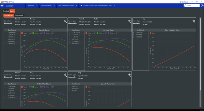
Curve tab

Cooling Mode sub tab
Capacity Curve
This biquadratic curve shows the percentage of full cooling capacity as a function of the condenser fluid temperature and the leaving chilled water temperature. Inputs consists of two independent variables, six coefficients, and min and max values for each of the independent variables. The equation for the capacity curve is:

Where:
Z = Cooling Capacity
C1 to C6 = coefficients
X = Condenser temperature
Y = Chilled Water Temperature
The curve has the following fields:
|
X Axis:
|
Condenser fluid temperature (°F, °C). Depending on the input for Condenser Temperature Type on the product’s tab, this axis will be either the Leaving or Entering Condenser Fluid temperature.
|
|
Y Axis:
|
Cooling Capacity (%).
|
|
Tchw,l Min / Max :
|
Minimum and maximum temperature values (°F, °C) for the Chilled water leaving temperature variable. These values determine the three chilled water temperatures plotted, one is the maximum, one is the minimum and the last one is the midpoint between them.
|
|
Tcond,l Min / Max:
|
Minimum and Maximum temperature values (°F, °C) for the Condenser Temperature variable.
|
Fuel Input Curve
This biquadratic curve represents the chiller’s fuel consumption at full load as a function of the condenser fluid temperature and the leaving chilled water temperature. Inputs consists of two independent variables, six coefficients, and min and max values for each of the independent variables. The equation for the capacity curve is:
Where:
Z = Fuel Consumption
C1 to C6 = coefficients
X = Condenser temperature
Y = Chilled Water Temperature
The curve has the following fields:
|
X Axis:
|
Condenser fluid temperature (°F, °C). Depending on the input for Condenser Temperature Type on the product’s tab, this axis will be either the Leaving or Entering Condenser Fluid temperature.
|
|
Y Axis:
|
Fuel Consumption (%).
|
|
Tchw,l Min / Max :
|
Minimum and maximum temperature values (°F, °C) for the Chilled water leaving temperature variable. These values determine the three chilled water temperatures plotted, one is the maximum, one is the minimum and the last one is the midpoint between them.
|
|
Tcond,l Min / Max:
|
Minimum and Maximum temperature values (°F, °C) for the Condenser Temperature variable.
|
Fuel Capacity Curve
This quadratic curve represents the chiller’s fuel consumption at part load with operating temperatures at design values. The equation for the Fuel Capacity Curve is:
Where:
y = Fuel Consumption
C1 to C3 = coefficients
X = Part Load
The curve has the following fields:
|
X Axis:
|
Part Load (%)
|
|
Y Axis:
|
Fuel Consumption (%).
|
|
Cycle Point:
|
Represents the percentage (%) of full load capacity at which the equipment will turn on and off (cycle) to satisfy the load.
|
Ambient Relief Curve
This biquadratic curve represents chiller’s electric consumption at full load as a function of the condenser fluid temperature and the leaving chilled water temperature. Inputs consists of two independent variables, six coefficients, and min and max values for each of the independent variables. The equation for the capacity curve is:
Where:
Z = Chiller’s electric consumption (%)
C1 to C6 = coefficients
X = Condenser temperature
Y = Chilled Water Temperature
The curve has the following fields:
|
X Axis:
|
Condenser fluid temperature (°F, °C). Depending on the input for Condenser Temperature Type on the product’s tab, this axis will be either the Leaving or Entering Condenser Fluid temperature.
|
|
Y Axis:
|
Chiller's electric consumption (%).
|
|
Tchw,l Min / Max :
|
Minimum and maximum temperature values (°F, °C) for the Chilled water leaving temperature variable. These values determine the three chilled water temperatures plotted, one is the maximum, one is the minimum and the last one is the midpoint between them.
|
|
Tcond,l Min / Max:
|
Minimum and Maximum temperature values (°F, °C) for the Condenser Temperature variable.
|
Electric Power Curve (Capacity Power Curve)
This quadratic curve represents the chiller’s electric consumption at part load with operating temperatures at design values.
The equation for the Fuel Capacity Curve is:
Where:
y = Chiller’s electric consumption (%)
C1 to C3 = coefficients
X = Part Load
The curve has the following fields:
|
X Axis:
|
Part Load (%)
|
|
Y Axis:
|
Electric Consumption (%).
|
|
Cycle Point:
|
Represents the percentage (%) of full load capacity at which the equipment will turn on and off (cycle) to satisfy the load.
|
Heating Mode sub tab
Heating Capacity Power Curve
This quadratic curve represents the chiller’s heating capacity as a function of its cooling capacity when the chiller is simultaneously cooling and heating.
The equation for the Heating-Cooling Capacity Curve is:
Where:
y = Heating Capacity (%)
C1 to C3 = coefficients
X = Cooling Capacity (%)
The curve has the following fields:
|
X Axis:
|
Cooling Capacity (%)
|
|
Y Axis:
|
Heating Capacity (%).
|
|
Capacity Min/Max:
|
Minimum and maximum Cooling capacity of the chiller.
|
Heating Fuel Power Curve
This quadratic curve represents the chiller’s fuel consumption as the heating load varies when the chiller is operating only as heater.
The equation for the Heating Fuel Power Curve is:
Where:
y = Fuel Consumption during heating mode (%)
C1 to C3 = coefficients
X = Heating Part Load (%)
The curve has the following fields:
|
X Axis:
|
Heating Part Load (%)
|
|
Y Axis:
|
Fuel Consumption during heating mode (%).
|
|
Load Min/Max:
|
Minimum and maximum Heating load of the chiller.
|